Technology Forecasting Methods: Wright’s Law

What is Wright’s Law?

As discussed in our previous post, the first of the technology forecasting formulations was Wright’s Law, posed in 1936. Similar to previous concepts used in psychology to describe the effect of learning, Wright used the learning effect to describe production costs in the aircraft industry.

Simply put, Wright’s Law says that as experience producing an item increases, the cost or time required to produce it decreases.

Learning curves of individual sub-technologies are often steep at the start as initial technical problems are grappled with, before leveling out as problems are solved and that specific solution implementation is more or less solved. Paradoxically, as described by both the Jevons Paradox and the Khazzoom-Brookes postulate, this often correlates with increased economic activity-it also often correlates with increasing technological capabilities as a whole.

When forecasting a more abtract concept such as computing power or (more easily) transistors on a chip, it is likely that it is comprised of multiple specific learning curves, and understanding this is important when interpreting data sets. Manufacturing processes have changed as transistors have shrank, and each of those had their own Wright learning curve.

While we’ll cover learning curves more in depth in a later post, what this meant is that as the production of a technology progressed and more units increased, the overall cost or time (often interchangeable) dropped correspondingly. Unlike Moore’s Law, it is not strictly time dependent, and unlike Goddard’s Law, it builds in effects of previous years due to be cumulative.

Mathematical Formulation

The mathematical formulation of Wright’s law is expressed where Y, the time or cost of one unit of production, is a function of number of units produced, time to produce each unit, and a ‘learning curve’ value.

• Y is the cumulative average time or cost per unit, expected to go down as workers and capital gain familiarity with the technology being produced.
• X is the cumulative number of units produced.
• a is the time or cost required to produce the first unit.
• b is the slope of the learning function when plotted on log-log paper.

b is slightly more complicated. As an example, for an 80% learning curve, the calculation for b would take the form

 

What does this look like in practice? As an example, say there’s some technological widget (a final device or component) that takes $500 to produce the first batch of units. If there’s a learning curve of 80%, it means that every time the cumulative output is doubled, the cumulative average cost goes down by 20%.

We can plug this into our equation. While it’s unlikely we’ll know what the learning curve is ahead of time, it’s a good proof of concept. So we plug in the starting price a ($500), the number of units produced X (1), and the learning curve value we calculated above, b (80%, or -.32).

Here’s a link to Wolfram Alpha so you can play with it yourself if you want, but the answer is total cost Y is $500. If it took $500 to produce the first unit, how much does it cost to produce the second unit? Well, the starting price and learning curve aren’t changing, but our output is doubling.

The answer isn’t quite $400, because we truncated the learning curve for ease.

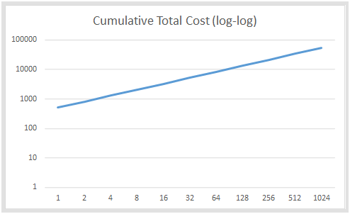
This formulation is easy for calculating how the cost changes as more units are produced. To calculate the cumulative cost, both sides of the equation are multiplied by X, yielding a new equation.

In our case, this means the equation for the 1000th unit would be

This means each unit would cost $54.82.

To help you visualize, we plotted out four graphs with the above numbers for the first 1024 (base 2 is easy!) units produced.

Context

Wright’s Law was the first of the major technology forecasting laws to emerging, and in turn inspired both Moore’s Law and Goddard’s Law, with a large volume of literature following it. We denote here the term ‘Wright’s Law’ as a comparison to Moore’s Law-in literature, it is more likely to simply be referred to as an experience curve, or experience curve analysis after it’s popularization by Boston Consulting Group in the 60s and 70s.

When examined by the survey of forecasting methods discussed in the previous post in this series (Overview), it was the most accurate of the implemented laws.

It’s important to note, however, that there is a body of history to its application to business and economic consultant, and limitations to its application. This doesn’t magically solve issues in the ability to know what sort of technologies will happen, but is more a statement in how production costs tend to change on large scales as time passes and production increases.

A number of criticisms have been levied against the use of experience curve methodologies for specific implementations, and using it blindly without understanding the situation can lead to a critical failure. Regardless, it remains an incredibly popular methodology in economic analysis.

Moving forward, we will examine Moore’s Law, how Wright’s Law compares to it, and the sort of obstacles it has seemingly overcome.